From Euclidean to Geometric ML

Perceptron & Curse of Dimensionality

Perceptron: \(y = \mathrm{sign}(w^T x + b)\)
Universal Approximation: 2-layer perceptrons approximate any continuous function
Curse of Dimensionality: to approximate \(f:\mathbb R^d\to\mathbb R\) within \(\varepsilon\), need \(O(\varepsilon^{-d})\) samples

Geometric Priors

Signals: \(x: \Omega \to \mathcal X\)
Symmetry group \(\mathcal G\) acting on domain \(\Omega\)

• Invariance (classification): \(f(\rho(g) x) = f(x)\)
• Equivariance (segmentation): \(f(\rho(g) x) = \rho(g) f(x)\)
  Scale separation: coarse-graining \(P:\Omega\to\Omega'\), \(f\approx f'\circ P\)

Geometric Deep Learning Blueprint

Architecture	Domain	Symmetry Group
CNN	Grid: \(\mathbb Z^n\)	Translations
Spherical CNN	Sphere: \(S^2\)	Rotations \(SO(3)\)
Intrinsic / Mesh CNN	Manifold	Isometry \(Iso(\Omega)\) / Gauge Symmetry \(SO(2)\)
GNN	Graph	Permutation \(\Sigma_n\)
DeepSets / Transformer	Set	Permutation \(\Sigma_n\)
Transformer	Complete Graph	Permutation \(\Sigma_n\)
LSTM	1D Grid: \(\mathbb Z\)	Time-warping

Graphs & Graph Neural Networks

Graph = Systems of Relations and Interactions

Graph \(G=(\mathcal V,\mathcal E)\)
Node features \(X\in\mathbb R^{n\times F}\)
Adjacency \(A\in\{0,1\}^{n\times n}\)
Permutation invariance: \(f(PX,PAP^T)=f(X,A)\)
Permutation equivariance: \(F(PX,PAP^T)=P\,F(X,A)\)

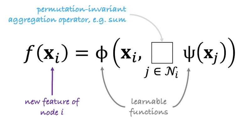
General Graph Function

1. For each node \(i\), gather neighbor features \(\{x_j:j\in\mathcal N(i)\}\)
2. Aggregate via permutation-invariant op (sum, mean, max)
3. Update: \(f(x_i) = \phi\bigl(x_i,\fbox{ }_{j\in\mathcal N(i)}\Psi(x_j)\bigr)\)
   

“Flavors” of GNNs

Convolutional (GCN): \(f(x_i) = \phi\bigl(x_i,\mathrm{AGG}_{j\in\mathcal N(i)}c_{ij}\Psi(x_j)\bigr)\), where \(c_{ij}\) is importance of node \(j\) to the representation of \(i\) Attentional (GAT): \(f(x_i) = \phi\bigl(x_i,\mathrm{AGG}_{j\in\mathcal N(i)}\alpha(x_i,x_j)\Psi(x_j)\bigr)\)
Message Passing (MPNN): \(f(x_i) = \phi\bigl(x_i,\mathrm{AGG}_{j\in\mathcal N(i)}\Psi(x_i,x_j)\bigr)\)

Typical Graph Tasks

Node classification: \(\hat y_i = \mathrm{softmax}(z_i)\)
Graph classification: \(\hat y = \mathrm{softmax}\bigl(\sum_i z_i\bigr)\) Link prediction: \(\displaystyle p(A_{ij}=1) = \sigma\bigl(z_i^\top z_j\bigr).\)

Special Cases

DeepSets / PointNet: per-element MLP + global max-pool
Transformers: complete graph + self-attention
LSTMs: sequential message passing

Graph Convolutional Networks (GCNs)

• Core idea:
  Each node updates its representation by combining (a) its own feature vector and (b) the (normalized) features of its neighbors, then applying a non-linearity.
• update rule: \(\mathbf{h}_i^{(l+1)} \;=\; \sigma\Bigl( \mathbf{h}_i^{(l)}\,\mathbf{W}_0^{(l)} \;+\; \sum_{j \in \mathcal{N}_i} \frac{1}{c_{ij}}\;\mathbf{h}_j^{(l)}\,\mathbf{W}_1^{(l)} \Bigr)\)
  • \(\mathcal{N}_i\): neighborhood of node ii
  • \(c_{ij}\): normalization constant (fixed or trainable)
  • \(\sigma\): activation function
• Desirable properties:
  • Shared weights across all nodes
  • Invariance to node-index permutations
  • Linear in the number of edges O(E)
  • Works in both transductive (full-graph) and inductive (new-node) settings
• Limitations:
  • Deep GCNs need gating or residual connections to avoid vanishing gradients
  • Edge features aren’t directly incorporated (only via neighbor aggregation)
• Scalability tip:
  • “Subsample messages” (e.g. GraphSAGE-style neighbor sampling) to handle large graphs

Edge-Embedding GNNs

Architecture

1. Node→Edge (“v→e”):
   • For each edge (i,j), compute an edge embedding \(\mathbf{h}_{(i,j)}^l \;=\; f_e^l\bigl([\mathbf{h}_i^l,\;\mathbf{h}_j^l,\;\mathbf{x}_{(i,j)}]\bigr)\)
     via an MLP that takes the two endpoint node embeddings plus any edge features.
2. Edge→Node (“e→v”):
   • For each node jj, aggregate its incoming edge embeddings and combine with its own features: \(\mathbf{h}_j^{\,l+1} \;=\; f_v^l\Bigl(\bigl[\!\!\sum_{i\in\mathcal{N}_j}\!\mathbf{h}_{(i,j)}^l,\;\mathbf{x}_j\bigr]\Bigr)\)
   • Another MLP produces the updated node embedding. Pros - Explicit edge features: Naturally incorporates edge attributes - Greater expressivity: More powerful than vanilla GCNs - Very general: Captures arbitrary node-edge interactions - Sparse ops possible: Can leverage sparse matrix routines for efficiency Cons - Memory overhead: Must store all intermediate edge embeddings - Hard to subsample: Neighborhood sampling breaks the two-stage flow - Scales poorly: In practice, typically limited to smaller graphs

Graph Attention Networks (GAT)

Core Mechanism

1. Attention Coefficients
   • For each edge (i,j)(i,j), compute \(e_{ij} = \text{LeakyReLU}\bigl(\mathbf{a}^T [\,\mathbf{W}\mathbf{h}_i \,\|\, \mathbf{W}\mathbf{h}_j]\bigr)\)
   • Normalize via softmax over \(j\in\mathcal{N}_i\): \(\alpha_{ij} = \frac{\exp(e_{ij})}{\sum_{k\in\mathcal{N}_i}\exp(e_{ik})}\)
2. Node Update
   • Multi-head attention (KK heads): \(\mathbf{h}_i' = \sigma\Bigl(\tfrac{1}{K}\sum_{k=1}^K \sum_{j\in\mathcal{N}_i}\alpha_{ij}^k\,\mathbf{W}^k\mathbf{h}_j\Bigr)\)
   • Optionally concatenate instead of averaging, then apply nonlinearity σ\sigma.

Pros

• No edge-state storage (with dot-product attention)
• Balance of speed & expressivity:Slower than GCNs, but faster than full edge-embedding GNNs Cons
• Less expressive than architectures with explicit edge embeddings
• Optimization challenges: attention weights can be harder to train

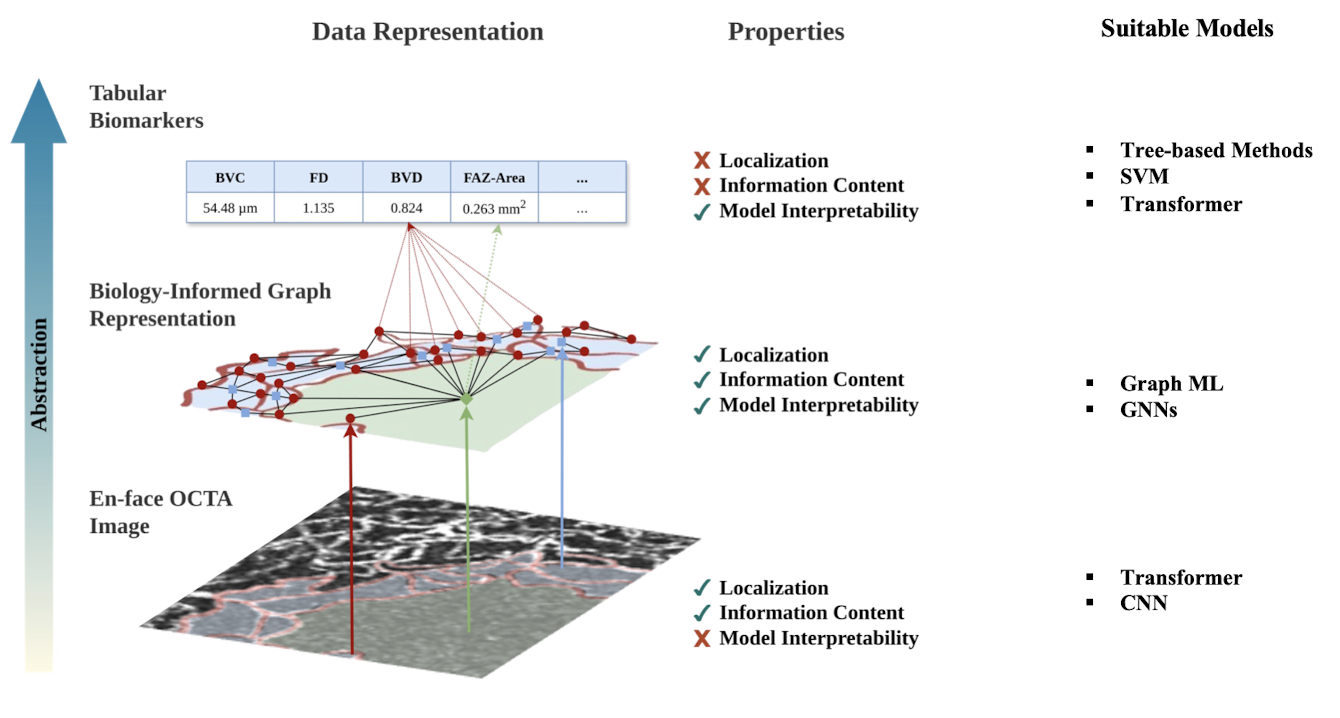
Applications in Medicine

Supervised Classification

Task: healthy vs. diseased (e.g., diabetic retinopathy)
Models: tree-based, SVM, CNN, Transformers, GNNs

Population Graphs for Brain Imaging

Assume N patient with

• imaging (e.g. resting-state fMRI or structural MRI)
• non-imaging (e.g. age, gender, acquisition site, etc.). Goal: assign to each patient a label l ∈L describing the corresponding subject’s disease state (e.g. control or diseased). Population is modelled as a sparse graph \(G=\{V,E,W\}\) Nodes: subjects with imaging features (e.g., connectivity, volumes)
  Edges: phenotypic similarity (age, gender, site)
  GCN pipeline:
  1. Build \(G=(V,E,W)\) where
     \(\displaystyle W_{vw} = \mathrm{Sim}(S_v,S_w)\times\sum_h\rho(M_h(v),M_h(w))\)
  2. Stack graph-conv+ReLU layers
  3. Softmax output per node, train with cross-entropy

Case Studies

ABIDE: ASD vs. controls, feature selection (RFE, PCA, AE, MLP)
ADNI: MCI → Alzheimer’s prediction, longitudinal data

• Multi-modal fusion: integrate imaging + non-imaging data
• Label propagation: leverage graph structure for semi-supervised learning
• Longitudinal modeling: handle repeat scans via intra-subject edges