Problem Formulation

Forward model \(y = A x + n\)

• Goal: recover \(x\) from noisy measurements \(y\)
• Applications: inpainting, deblurring, denoising, super-resolution, reconstruction, registration

Classical Approach

Least-squares problem

\(\arg\min_x \mathcal{D}(Ax,y) = \arg\min_x\tfrac12\|A x - y\|^2\) solution \(\hat{x}= (A^T A)^{-1}A^T y\)

ill-posed problem: similar y can leads to wildly different solutions

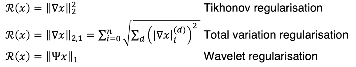
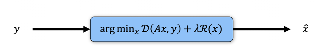
Regularization

\(\arg\min_x \mathcal{D}(Ax,y)+\lambda\mathcal{R}(x)\) where \(\mathcal{D}(Ax,y)\) data consistency term, \(\mathcal{R}(x)\) regularisation term (encoding prior knowledge on \(x\)), \(\lambda\) regularisation parameter.

Common regularisers

ML Approach

Instead of choosing \(\mathcal{R}\) a-priori based on a simple model of image, learn \(\mathcal{R}\) from training data.

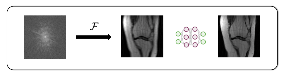
Forward & Inverse Models

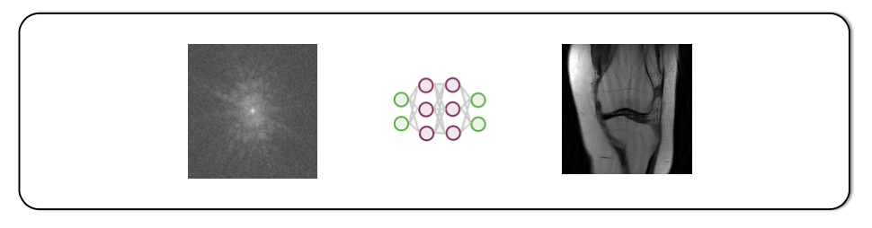
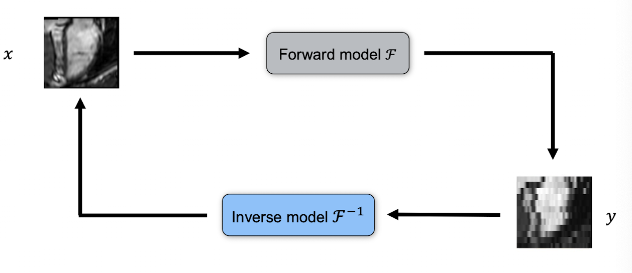Inverse model \(\mathcal{F}_\phi^{-1}\): directly map \(y\to x\) via a trained network.

Method Taxonomy

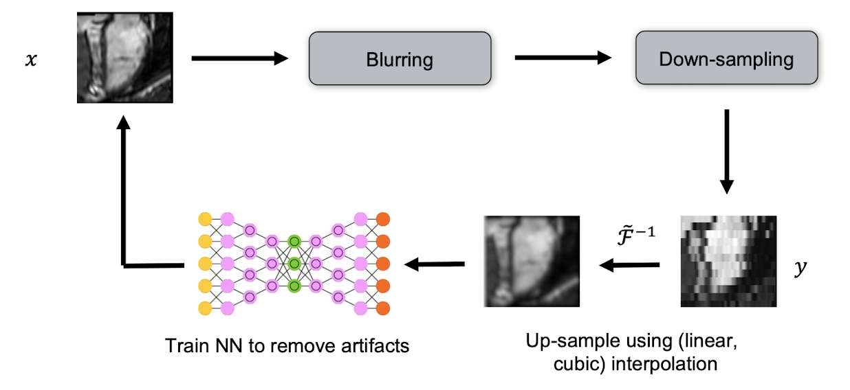
Model-agnostic

• Ignore \(A\), learn \(y\to x\) directly
• Example: Up-sampling

Decoupled

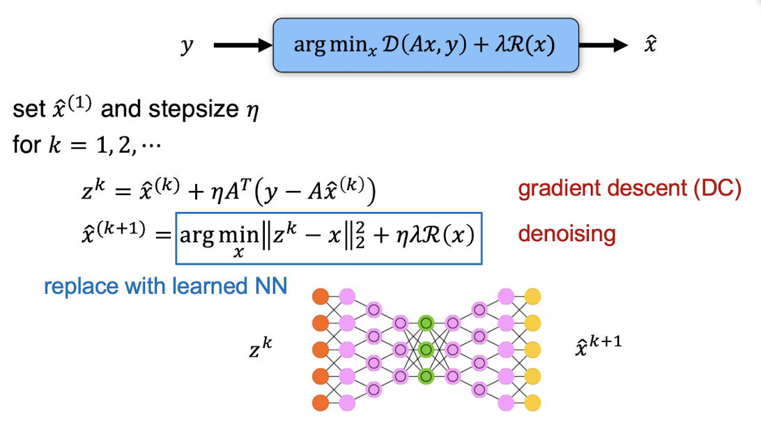
• Learn denoiser or prior, then plug into classical solver (plug-and-play)
• Example: Deep proximal gradient -> unroll proximal gradient steps, replace proximal operator with learned denoiser
  
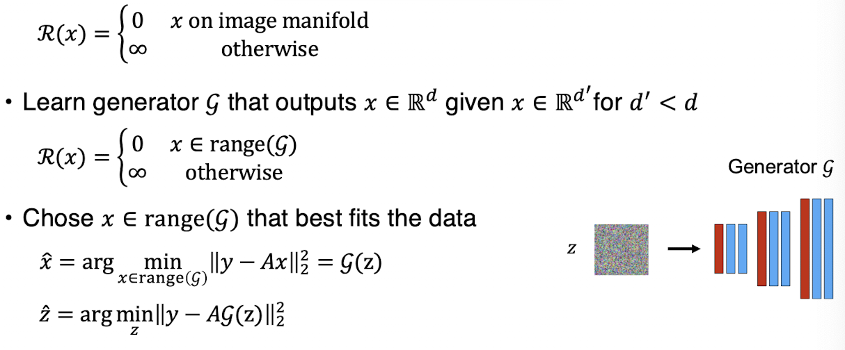
• Example: GANs -> constrain \(x\) to lie in generator manifold \(\mathcal G(z)\), solve \(\min_z\|y - A\mathcal G(z)\|\)
  

Unrolled Optimization

• Embed iterative solver steps into a network and learn updates
• Example: Gradient Descent Networks -> unroll gradient descent and learn components Assume R(x) is differentiable

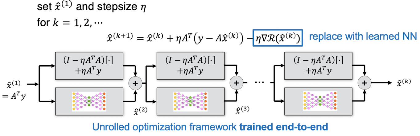
Image Super-Resolution

Problem formulation: Upsample low-resolution (LR) image to high-resolution (HR or SR)

Common Super-Resolution Frameworks

Post-upsampling: (interpolate)

• directly upsample LR image into SR with learnable upsampling layers
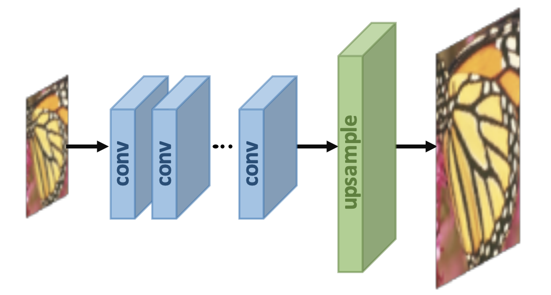
• fast, low memory
• has to learn entire upsampling pipeline
• limited to a specific up-sampling factor

Pre-upsampling: two-stage process (interpolate then refine)

• First use traditional upsampling algorithm (e.g. linear interpolation) to obtain SR images; Then refining upsampled using a deep neural network (usually a CNN)
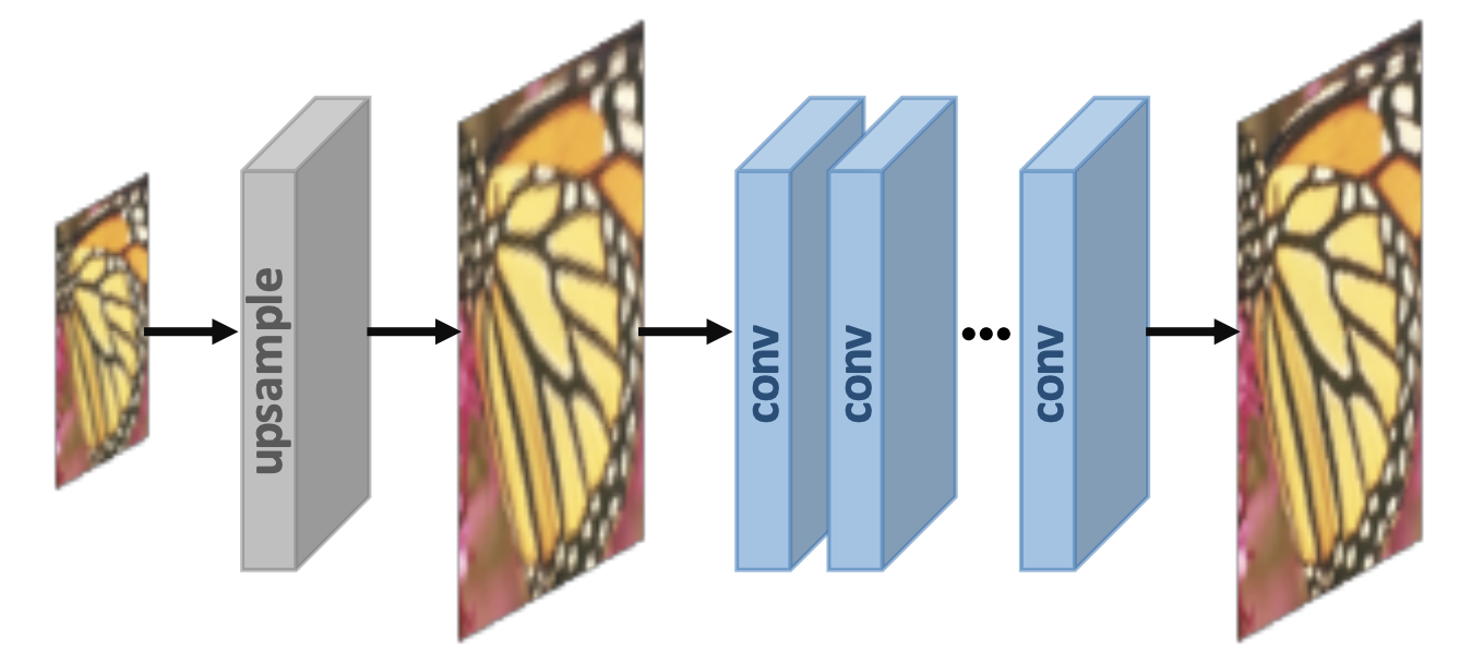
• flexible scaling,
• higher compute and memory

Progressive Upsampling: multi-stage process (gradual resolution increase)

• Use a cascade of CNNs to progressively reconstruct higher-resolution images.
• At each stage, the images are upsampled to higher resolution and refined by CNNs
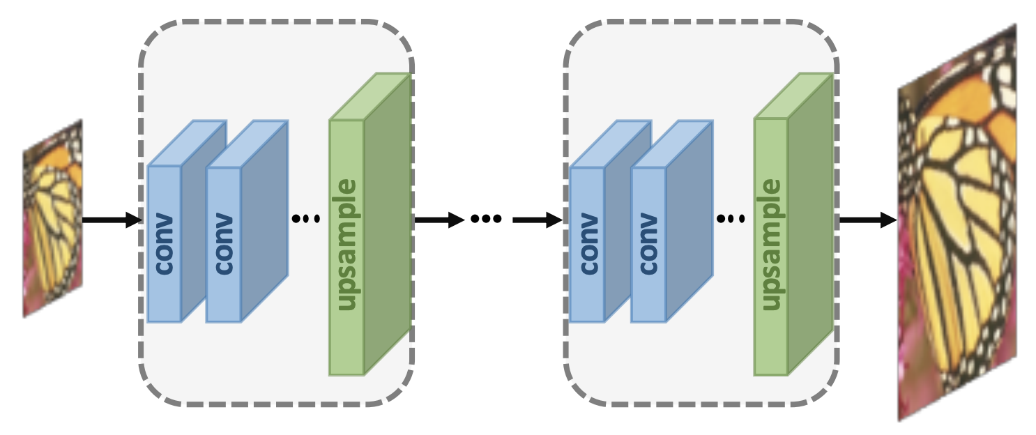
• Decomposes complex task into simple tasks
• Reasonable efficiency
• Sometimes difficult to train very deep models

Iterative Back-Projection: alternate for error feedback

• Alternate between upsampling and downsampling (back-projection) operations

• Mutually connected up- and down-sampling stages

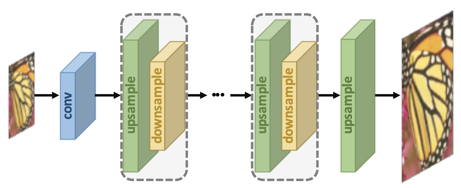
• Superior performance as it allows error feedback
• Easier training of deep networks

Losses pixel-wise (L1/L2, Huber), perceptual (VGG features), total variation, adversarial (GAN)

Deep Image Prior

• Idea: a randomly initialized network \(\Psi(z;w)\) fits a single image by optimizing \(w\) on observed pixels
• Applications: denoising, inpainting (solve \(\min_w\|\,(m\odot x) - (m\odot \Psi(z;w))\|^2\))

Image Reconstruction

CT

• high-contrast; high spatial resolution; fast acqiusition; but ionising radiation
• sinogram \(\to\) image via Radon inverse; ill-posed inverse problem under sparse views;
• under-sampled reconstruction to reduce radiation

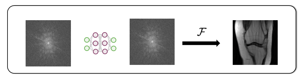
MRI

• high-contrast; high spatial resolution; no ionising radiation; but slow acquisition process(problematic for moving objects)
• recover image from undersampled k-space (\(y = F x + n\)); aliasing correction needed
• Undersampling patterns:
  • low frequency only: blurring; loss of detail
  • regular cartesian: coherent wrap-around along PE direction
  • variable-density random: incoherent “noise-like” aliasing
  • radial: streaks from strong edges
  • spiral: off-resonance artifacts at sharpities
• Reconstruction approaches
  • interpolation in k-space
  • deblurring in image space
  • transform/operator learning